8. 2017 Denver Inversion
8.1. Model Configuration and Datasets
The case runs are initialized at 00z Oct 16, 2017 with 120 hours forecasting. The corresponding namelist options that need to be changed are listed below. The app uses ./xmlchange to change the runtime settings. The settings that need to be modified to set up the start date, start time, and run time are listed below.
./xmlchange RUN_STARTDATE=2017-10-16,START_TOD=0,STOP_OPTION=nhours,STOP_N=120
Initial condition (IC) files are created from GFS operational dataset in NEMSIO format. Sounding profiles can be downloaded from the University of Wyoming.
The GFS model EMC global workflow points to the most up-to-date GFS model development code. The GFS.v16.0.10 is tested in C768 (~13km) resolution and in 128 vertical levels. It uses two scripts, setup_expt_fcstonly.py and setup_workflow_fcstonly.py to set up the mode simulation date and case directories.
The case runs are initialized at 00z Oct 16, 2017 with 120 hours forecasting. The settings that need to be modified to set up the start date and directories are listed below.
./setup_expt_fcstonly.py --pslot 2017DNRInversion --configdir /PATH/TO/YOUR/GLOBAL/WORKFLOW/parm/config --idate 2017101600 --edate 2017101600 --res 768 --comrot /PATH/TO/YOUR/EXP/DIR/comrot --expdir /PATH/TO/YOUR/EXP/OUTPUT/expdir
The account and simulation duration time can be set up in /expdir/2017DNRInversion/config.base file.
./setup_workflow_fcstonly.py --expdir /PATH/TO/YOUR/OUTPUT/expdir/2017DNRInversion
Next step is to go to /expdir/2017DNRInversion to submit the run by
crontab 2017DNRInversion.crontab
8.2. Case Results
8.2.1. Skew-T Log-P Plot
The Skew-T Log-P plot is created using the script adapted from SHARPpy. The steps for using the SHARPpy scripting in Python programming language is here.
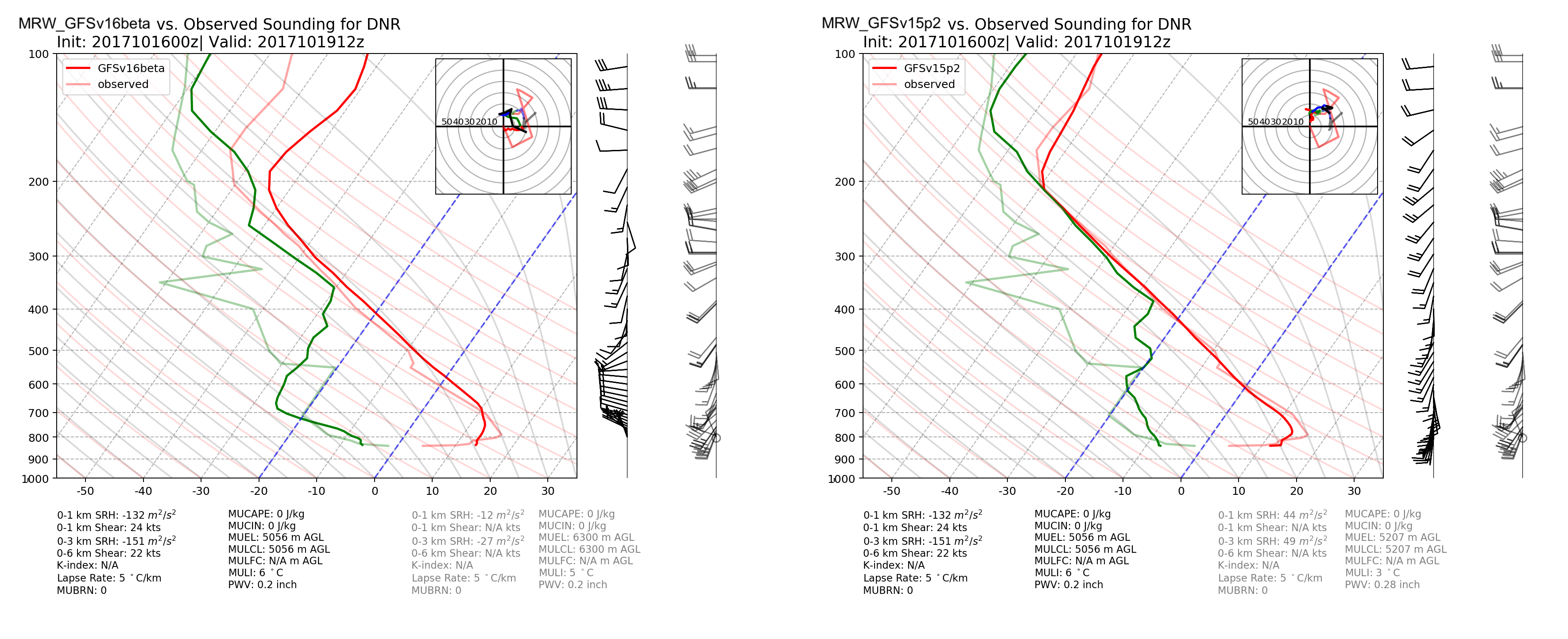
Skew-T Log-P plot from observed and simulated sounding profiles. Indices including K-index and lapse rate are shown in the bottom.
The two physics compsets, MRW_GFSv15p2 and MRW_GFSv16beta, underestimate the temperature inversion strength at 800 hPa with a warmer near surface temperature and a colder temperature at the top of inversion.
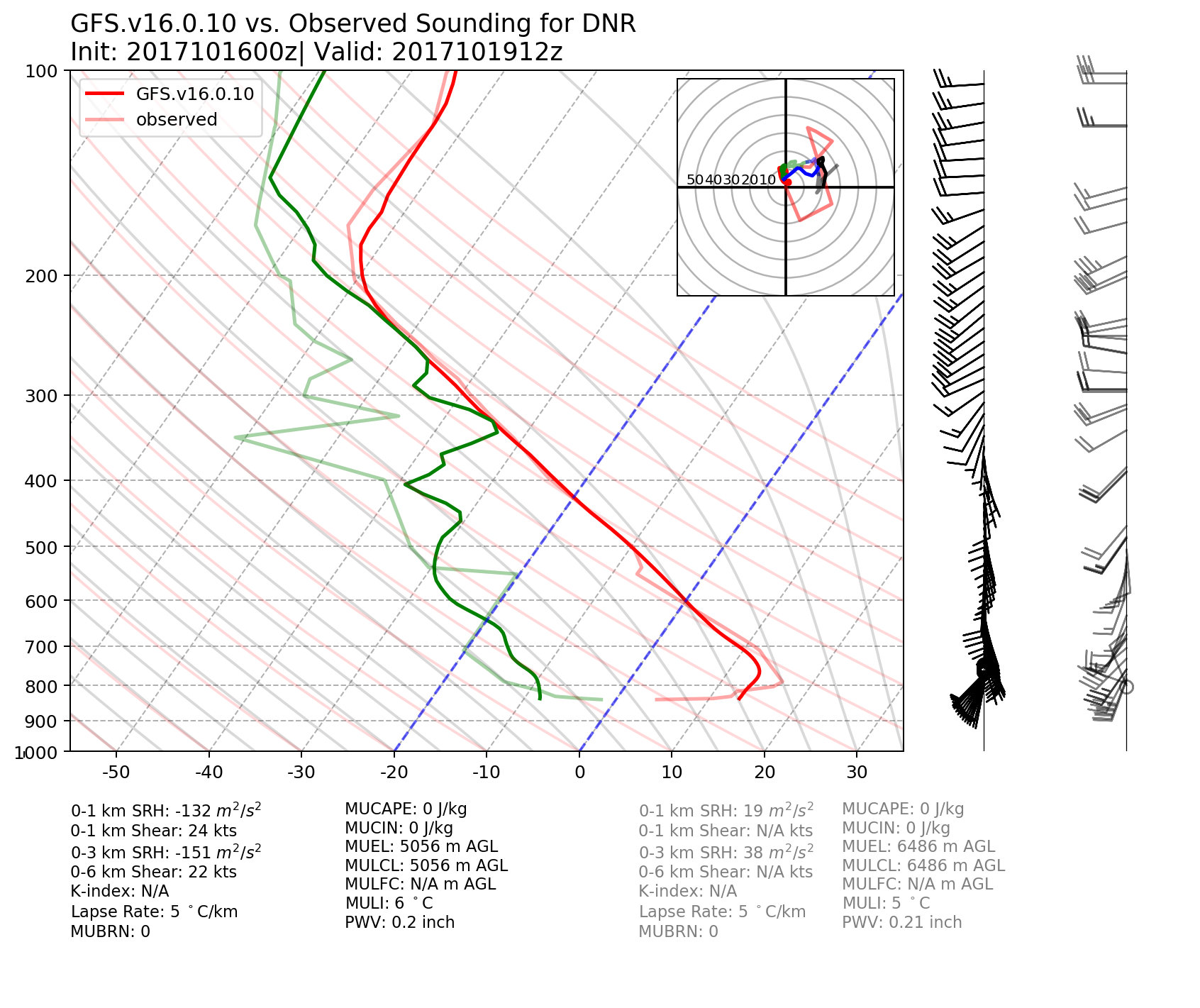
Skew-T Log-P plot from observed and simulated sounding profiles. Indices including K-index and lapse rate are shown in the bottom.
GFS.v16.0.10 underestimates the temperature inversion strength at 800 hPa with a warmer near surface temperature and a colder temperature at the top of inversion.
8.3. Summary and Discussion
The 2017 Denver Inversion results show that the GFS model lacks skills in forecasting the boundary layer temperature inversion for MRW_GFSv15p2, MRW_GFSv16beta, and GFS.v16.0.10, with a warmer near-surface temperature and a colder temperature at the top of the inversion.